Quickstart#
This is a concise introduction to pyathena, aimed mainly at new users.
Start by importing the necessary modules.
To use pyathena, add its directory to the PYTHONPATH environment variable in .bashrc or .bash_profile
export PYTHONPATH=/path/to/directory:$PYTHONPATH
Alternatively, you can dynamically add the path in your script or notebook.
import sys
sys.path.insert(0, '..')
import pyathena as pa

import numpy as np
import matplotlib as mpl
import matplotlib.pyplot as plt
import pandas as pd
import xarray as xr
LoadSim class#
The LoadSim class is the primary interface for handling Athena/Athena++ simulation data.
Use the help() function to access documentation for the class:
help(pa.LoadSim)
Pro Tip: Use class_or_func_name?, class_or_func_name??, help(class_or_func_name), or Shift+Tab in an interactive Python environment to view documentation, summaries, or source code.
Initialization#
Simulation Directory:
LoadSimuses thebasedirparameter to locate all output files (hst,hdf5,vtk, etc.).Save Directory: The
savdirparameter defines the directory for saving pickles and figures. If unspecified, it defaults tobasedir.Logger: A logger is attached to the
LoadSiminstance print out log messages. The verbosity can be adjusted by settingverbosetoTrue(equivalent"INFO") orFalse(equivalent"WARNING") or different levels of logging"DEBUG","INFO","WARNING","ERROR"(case insensitive). The default is set toFalse.Metadata : During the initialization,
FindFilesclass is initialized withinLoadSimand it tries to find the athinput file and (e.g.,athinput.runtime) or a file (e.g.,out.txt) where standard output is redirected to. It then reads in simulations parameters and code configuration and saves results to a dictionary of dictionaries,par, containing all information. Other important metadata include information about the computational domain (domain), the date and time when code was configured (config_time).Finding files : Find output files based on the information available from par. The
find_files()method can be called to find file names (files) and lists of snapshot numbers (nums*) again. File formats includeAthena-TIGRESS :
hst,sn,zprof,vtk,starpar_vtk,rst,timeitTIGRIS :
hst,sn,zprof,hdf5,rst,loop_time/task_time
import sys
sys.path.insert(0, '..')
import pyathena as pa

basedir = '/tigress/changgoo/TIGRESS-NCR/R8_8pc_NCR.full.xy2048.eps0.0/'
s = pa.LoadSim(basedir, verbose=True)
[LoadSim-INFO] basedir: /tigress/changgoo/TIGRESS-NCR/R8_8pc_NCR.full.xy2048.eps0.0
[LoadSim-INFO] savdir: /tigress/changgoo/TIGRESS-NCR/R8_8pc_NCR.full.xy2048.eps0.0
[LoadSim-INFO] load_method: pyathena
[FindFiles-INFO] athinput: /tigress/changgoo/TIGRESS-NCR/R8_8pc_NCR.full.xy2048.eps0.0/out.txt
[FindFiles-INFO] athena_pp: False
[FindFiles-INFO] problem_id: R8_8pc_NCR
[FindFiles-INFO] vtk in tar: /tigress/changgoo/TIGRESS-NCR/R8_8pc_NCR.full.xy2048.eps0.0/vtk nums: 200-668
[FindFiles-INFO] hst: /tigress/changgoo/TIGRESS-NCR/R8_8pc_NCR.full.xy2048.eps0.0/hst/R8_8pc_NCR.hst
[FindFiles-INFO] sn: /tigress/changgoo/TIGRESS-NCR/R8_8pc_NCR.full.xy2048.eps0.0/hst/R8_8pc_NCR.sn
[FindFiles-INFO] zprof: /tigress/changgoo/TIGRESS-NCR/R8_8pc_NCR.full.xy2048.eps0.0/zprof nums: 200-668
[FindFiles-INFO] starpar_vtk: /tigress/changgoo/TIGRESS-NCR/R8_8pc_NCR.full.xy2048.eps0.0/starpar nums: 200-668
[FindFiles-INFO] rst: /tigress/changgoo/TIGRESS-NCR/R8_8pc_NCR.full.xy2048.eps0.0/rst/0010 nums: 10-34
[FindFiles-INFO] timeit: /tigress/changgoo/TIGRESS-NCR/R8_8pc_NCR.full.xy2048.eps0.0/timeit.txt
Attributes#
Print some (read-only) attributes of a LoadSim instance.
s.basedir
'/tigress/changgoo/TIGRESS-NCR/R8_8pc_NCR.full.xy2048.eps0.0'
s.basename
'R8_8pc_NCR.full.xy2048.eps0.0'
s.problem_id
'R8_8pc_NCR'
domain contains information about simulation domain
Nx: Number of cells
le/re: left/right edge
Lx: box size
dx: cell size
s.domain
{'Nx': array([128, 128, 768]),
 'ndim': 3,
 'le': array([ -512,  -512, -3072]),
 're': array([ 512,  512, 3072]),
 'Lx': array([1024, 1024, 6144]),
 'dx': array([8., 8., 8.]),
 'center': array([0., 0., 0.]),
 'time': None}
Date and time when the code is compiled
s.config_time
Timestamp('2022-05-18 14:19:25-0700', tz='US/Pacific')
par contains all input parameters and meta information
s.par.keys()
dict_keys(['job', 'log', 'output1', 'output2', 'output3', 'output4', 'output5', 'time', 'domain1', 'problem', 'feedback', 'cooling', 'opacity', 'radps', 'configure'])
s.par['configure'].keys()
dict_keys(['config_date', 'config_server', 'git_commit_ID', 'problem', 'gas', 'eq_state', 'nscalars', 'self-gravity', 'resistivity', 'viscosity', 'thermal_conduction', 'cooling', 'new_cooling', 'particles', 'sixray', 'radps', 'ionrad', 'lwrad', 'species_HI', 'species_H2', 'species_EL', 'species_CI', 'test_newcool', 'scalar_CL', 'star_particles', 'coord', 'special_relativity', 'order', 'flux', 'integrator', 'precision', 'write_ghost', 'mpi', 'H-correction', 'FFT', 'ShearingBox', 'RaytPlaneParallel', 'FARGO', 'FOFC', 'SMR'])
s.par['output2']
{'out_fmt': 'vtk',
 'out': 'prim',
 'dt': 1.0,
 'time': 201.0,
 'num': 200,
 'level': -1,
 'domain': -1,
 'id': 'out2',
 'new_output_directory': 1}
s.par['time']
{'selfg_no': 1,
 'cour_no': 0.3,
 'nlim': -1,
 'tlim': 700.0,
 'time': 200.0007,
 'nstep': 0}
s.par['problem']
{'gamma': 1.66666667,
 'surf': 12.0,
 'sz0': 10,
 'vturb': 10,
 'beta': 1,
 'qshear': 1.0,
 'Omega': 0.028,
 'SurfS': 42.0,
 'zstar': 245.0,
 'rhodm': 0.0064,
 'R0': 8000,
 'Sigma_SFR': 0.005,
 'Z_gas': 1.0,
 'Z_dust': 1.0,
 'xi_CR_amp': 1.0,
 'rho_crit': 1.0,
 'starpar_iacc': 0,
 'muH': 1.4,
 'Sigma_gas0': 10.0,
 'Sigma_SFR0': 0.0025,
 'tdecay_CR': -1.0}
Other attributes.
s.verbose # can be changed at any time
True
s.savdir
'/tigress/changgoo/TIGRESS-NCR/R8_8pc_NCR.full.xy2048.eps0.0'
s.load_method
'pyathena'
s.out_fmt
['hst', 'vtk', 'starpar_vtk', 'rst', 'zprof']
Finding files#
NOTE: If find_files() did not succeed in finding output files under basedir, check if the glob patterns s.ff.patterns are set appropriately. Update it and try again. For example, the history dump is found using the glob patterns /path_to_basedir/id0/*.hst first. If it fails, it searches again with /path_to_basedir/hst/*.hst, and then with /path_to_basedir/*.hst
s.files.keys()
dict_keys(['athinput', 'vtk_tar', 'hst', 'sn', 'zprof', 'starpar_vtk', 'rst', 'timeit'])
s.files['vtk_tar'][0], s.files['vtk_tar'][-1]
('/tigress/changgoo/TIGRESS-NCR/R8_8pc_NCR.full.xy2048.eps0.0/vtk/R8_8pc_NCR.0200.tar',
 '/tigress/changgoo/TIGRESS-NCR/R8_8pc_NCR.full.xy2048.eps0.0/vtk/R8_8pc_NCR.0668.tar')
s.nums[0], s.nums[-1], s.nums_starpar[0], s.nums_starpar[-1]
(200, 668, 200, 668)
type(s.ff)
pyathena.find_files.FindFiles
s.ff.patterns.keys()
dict_keys(['athinput', 'hst', 'sphst', 'sn', 'vtk', 'vtk_id0', 'vtk_tar', 'vtk_athenapp', 'hdf5', 'starpar_vtk', 'partab', 'parhst', 'zprof', 'timeit', 'looptime', 'tasktime', 'rst'])
s.ff.patterns['hst']
[('id0', '*.hst'), ('hst', '*.hst'), ('*.hst',)]
s.ff.patterns['vtk']
[('vtk', '*.????.vtk'), ('*.????.vtk',)]
s.ff.patterns['hdf5']
[('hdf5', '*.out?.?????.athdf'), ('*.out?.?????.athdf',)]
Units#
Simulations run with Athena-TIGRESS/TIGRIS use the following code units
TIGRESS-classic:
Mean particle mass per H: \(\mu_{\rm H} = 1.4271\)
\(1\;{code\_density} \leftrightarrow n_{\rm H} = 1 {\rm cm}^{-3}\)
Length : 1 pc
Velocity : 1 km/s
TIGRESS-NCR:
Mean particle mass per H: \(\mu_{\rm H} = 1.4\)
\(1\;{code\_density} \leftrightarrow n_{\rm H} = 1 {\rm cm}^{-3}\)
Length : 1 pc
Velocity : 1 km/s
TIGRIS with
"ism"units:Mean particle mass per H: \(\mu_{\rm H} = 1.4\)
\(1.4\;{code\_density} \leftrightarrow \rho = 1.4 m_{\rm H}\;{\rm cm}^{-3} \leftrightarrow n_{\rm H} = 1 {\rm cm}^{-3}\)
Length : 1 pc
Velocity : 1 km/s
u = s.u
# or
# u = pa.Units(kind='LV', muH=1.4)
Print code units (astropy Quantity)
type(s.u.time)
astropy.units.quantity.Quantity
s.u.time, s.u.mass, s.u.density, s.u.length, s.u.velocity, s.u.muH,
(<Quantity 3.08567758e+13 s>,
 <Quantity 0.03462449 solMass>,
 <Quantity 2.34335273e-24 g / cm3>,
 <Quantity 1. pc>,
 <Quantity 1. km / s>,
 1.4)
s.u.energy, s.u.energy_density, s.u.momentum, s.u.momentum_flux
(<Quantity 6.88476785e+41 erg>,
 <Quantity 2.34335273e-14 erg / cm3>,
 <Quantity 0.03462449 km solMass / s>,
 <Quantity 0.03541089 km solMass / (s yr kpc2)>)
Commonly used astronomical constants and units (plain numbers). Multiply them to convert quantities in code units to one in physical units. For example,
(code mass)*u.Msun = mass in Msun(code time)*u.Myr = time in Myr(code luminosity)*u.Lsun = luminosity in Lsun(code pressure)*u.pok = P/k_B in cm^-3 K
s.u.Msun, s.u.Myr, s.u.Lsun, s.u.pc, s.u.kms, s.u.pok
(0.034624490427439196,
 0.9777922216807893,
 5.82863455377993e-06,
 1.0,
 1.0,
 169.7283473776405)
VTK dump#
print(s.nums[0], s.nums[-1], len(s.nums)) # vtk file numbers in the directory
200 668 469
ds = s.load_vtk(num=s.nums[0])
[LoadSim-INFO] [load_vtk_tar]: R8_8pc_NCR.0200.tar. Time: 200.000700
ds.domain
{'all_grid_equal': True,
 'ngrid': 384,
 'le': array([ -512.,  -512., -3072.], dtype=float32),
 're': array([ 512.,  512., 3072.], dtype=float32),
 'dx': array([8., 8., 8.], dtype=float32),
 'Lx': array([1024., 1024., 6144.], dtype=float32),
 'center': array([0., 0., 0.], dtype=float32),
 'Nx': array([128, 128, 768]),
 'ndim': 3,
 'time': 200.0007}
ds.domain == s.domain
True
Note that domain['time'] is updated after reading loading a vtk file.
Field names#
The field_list contains all available variable names in vtk file, representing the raw data. The derived_field_list includes variables that are calculated based on those in the field_list, often expressed in more convenient units. Usually, fields in derived_field_list are in more convenient units. When in doubt, it is recommended to use variables from the field_list and calculate derived quantities yourself.
print(ds.field_list)
['density', 'velocity', 'pressure', 'cell_centered_B', 'gravitational_potential', 'temperature', 'heat_rate', 'cool_rate', 'net_cool_rate', 'CR_ionization_rate', 'rad_energy_density_PH', 'rad_energy_density_LW', 'rad_energy_density_PE', 'rad_energy_density_LW_diss', 'specific_scalar[0]', 'specific_scalar[1]', 'xHI', 'xH2', 'xe']
print(ds.derived_field_list)
['rho', 'nH', 'pok', 'r', 'vmag', 'vr', 'vx', 'vy', 'vz', 'cs', 'csound', 'Mr', 'Mr_abs', 'rhovr2ok', 'T', 'Td', 'cool_rate', 'heat_rate', 'net_cool_rate', 'Lambda_cool', 'nHLambda_cool', 'nHLambda_cool_net', 'Gamma_heat', 't_cool', 'vAmag', 'vAx', 'vAy', 'vAz', 'Bx', 'By', 'Bz', 'Bmag', 'nH2', '2nH2', 'xH2', '2xH2', 'nHI', 'xHI', 'nHII', 'xHII', 'nHn', 'xn', 'ne', 'nesq', 'xe', 'xCI', 'nCI', 'xOII', 'xCII', 'xCII_alt', 'xi_CR', 'T_alt', 'chi_PE', 'chi_LW', 'chi_FUV', 'Erad_LyC', 'Jphot_LyC', 'Uion', 'j_Halpha', 'Erad_FUV', 'heat_ratio', 'NHeff', 'heat_rate_HI_phot', 'heat_rate_H2_phot', 'heat_rate_dust_LyC', 'heat_rate_dust_FUV', 'heat_rate_dust_UV', 'psi_gr', 'eps_pe', 'Gamma_pe', 'chi_H2', 'chi_CI', 'fshld_H2', 'j_X']
ds.dirname, ds.ext
('/tigress/changgoo/TIGRESS-NCR/R8_8pc_NCR.full.xy2048.eps0.0/vtk', 'tar')
Read 3d data cubes#
With xarray=True option (default is True), read dataset as a xarray DataSet.
See http://xarray.pydata.org/en/stable/quick-overview.html for a quick overview of xarray.
help(ds.get_field) # Note: setting (le, re) manually may not work as intended
Help on method get_field in module pyathena.io.read_vtk:

get_field(field='density', le=None, re=None, as_xarray=True) method of pyathena.io.read_vtk_tar.AthenaDataSetTar instance
    Read 3d fields data.

    Parameters
    ----------
    field : (list of) string
        The name of the field(s) to be read.
    le : sequence of floats
       Left edge. Default value is the domain left edge.
    re : sequence of floats
       Right edge. Default value is the domain right edge.
    as_xarray : bool
       If True, returns results as an xarray Dataset. If False, returns a
       dictionary containing numpy arrays. Default value is True.

    Returns
    -------
    dat : xarray dataset
        An xarray dataset containing fields.
dat = ds.get_field(['nH', 'pok', 'T'])
Indexing follows the convention of the Athena code (k,j,i): for scalar fields, the innermost (fastest running) index is the x-direction, while the outermost index is the z-direction
dat['nH'].shape
(768, 128, 128)
dat
<xarray.Dataset>
Dimensions:  (x: 128, y: 128, z: 768)
Coordinates:
  * x        (x) float64 -508.0 -500.0 -492.0 -484.0 ... 484.0 492.0 500.0 508.0
  * y        (y) float64 -508.0 -500.0 -492.0 -484.0 ... 484.0 492.0 500.0 508.0
  * z        (z) float64 -3.068e+03 -3.06e+03 -3.052e+03 ... 3.06e+03 3.068e+03
Data variables:
    nH       (z, y, x) float32 0.0001338 0.0001325 ... 0.0003592 0.0003528
    T        (z, y, x) float32 2.277e+06 2.316e+06 ... 2.397e+06 2.451e+06
    pok      (z, y, x) float32 700.5 705.4 707.3 ... 1.98e+03 1.988e+03
Attributes:
    all_grid_equal:  True
    num:             200
    ngrid:           384
    le:              [ -512.  -512. -3072.]
    re:              [ 512.  512. 3072.]
    dx:              [8. 8. 8.]
    Lx:              [1024. 1024. 6144.]
    center:          [0. 0. 0.]
    Nx:              [128 128 768]
    ndim:            3
    time:            200.0007
dfi: {'rho': {'field_dep': ['density'], 'func': <function set...dat.x
<xarray.DataArray 'x' (x: 128)>
array([-508., -500., -492., -484., -476., -468., -460., -452., -444., -436.,
       -428., -420., -412., -404., -396., -388., -380., -372., -364., -356.,
       -348., -340., -332., -324., -316., -308., -300., -292., -284., -276.,
       -268., -260., -252., -244., -236., -228., -220., -212., -204., -196.,
       -188., -180., -172., -164., -156., -148., -140., -132., -124., -116.,
       -108., -100.,  -92.,  -84.,  -76.,  -68.,  -60.,  -52.,  -44.,  -36.,
        -28.,  -20.,  -12.,   -4.,    4.,   12.,   20.,   28.,   36.,   44.,
         52.,   60.,   68.,   76.,   84.,   92.,  100.,  108.,  116.,  124.,
        132.,  140.,  148.,  156.,  164.,  172.,  180.,  188.,  196.,  204.,
        212.,  220.,  228.,  236.,  244.,  252.,  260.,  268.,  276.,  284.,
        292.,  300.,  308.,  316.,  324.,  332.,  340.,  348.,  356.,  364.,
        372.,  380.,  388.,  396.,  404.,  412.,  420.,  428.,  436.,  444.,
        452.,  460.,  468.,  476.,  484.,  492.,  500.,  508.])
Coordinates:
* x (x) float64 -508.0 -500.0 -492.0 -484.0 ... 484.0 492.0 500.0 508.0Mean value of nH, pressure/kB at the midplane
dat.sel(z=0, method='nearest').mean()
<xarray.Dataset>
Dimensions:  ()
Coordinates:
    z        float64 4.0
Data variables:
    nH       float32 0.8858
    T        float32 6.296e+05
pok float32 9.153e+03Slice plots#
Use
dat.dfiors.dfi(derived field info) to set plot argumentsSee also https://docs.xarray.dev/en/latest/generated/xarray.plot.imshow.html
dat.dfi['nH']
{'field_dep': ['density'],
 'func': <function pyathena.fields.fields.set_derived_fields_def.<locals>._nH(d, u)>,
 'label': '$n_{\\rm H}\\;[{\\rm cm^{-3}}]$',
 'norm': <matplotlib.colors.LogNorm at 0x14a046191780>,
 'vminmax': (0.001, 10000.0),
 'cmap': 'Spectral_r',
 'scale': 'log',
 'take_log': True,
 'imshow_args': {'norm': <matplotlib.colors.LogNorm at 0x14a046191780>,
  'cmap': 'Spectral_r',
  'cbar_kwargs': {'label': '$n_{\\rm H}\\;[{\\rm cm^{-3}}]$'}}}
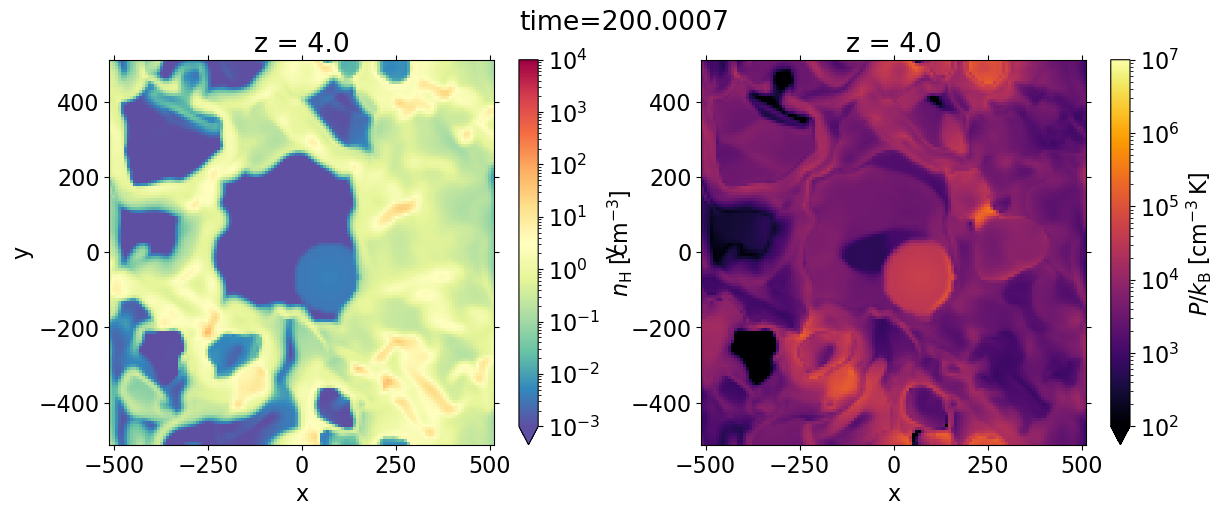
fig, axes = plt.subplots(1, 2, figsize=(14, 5))
dat['nH'].sel(z=0, method='nearest').plot.imshow(ax=axes[0], **dat.dfi['nH']['imshow_args'])
dat['pok'].sel(z=0, method='nearest').plot.imshow(ax=axes[1], **dat.dfi['pok']['imshow_args'])
plt.setp(axes, aspect='equal')
plt.suptitle(f'time={dat.time}')
Text(0.5, 0.98, 'time=200.0007')
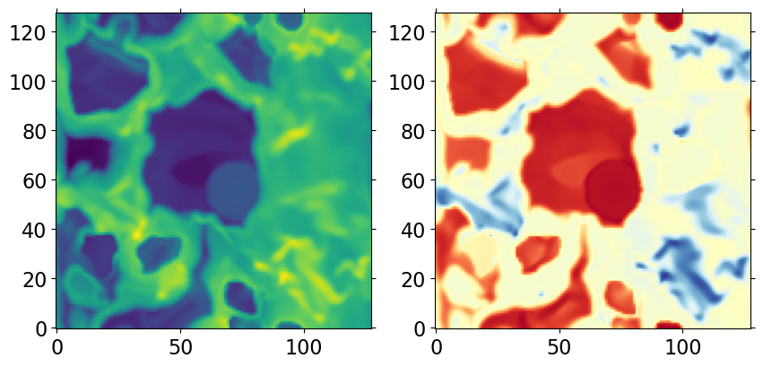
Another example: plot slice of density and temperature at z=0
d = ds.get_field(['nH', 'T'])
from pyathena.plt_tools.cmap_shift import cmap_shift
iz = ds.domain['Nx'][2] // 2
fig, axes = plt.subplots(1, 2, figsize=(10,5))
cmap_temp = cmap_shift(mpl.cm.RdYlBu_r, midpoint=3.0/7.0)
axes[0].imshow(d['nH'][iz,:,:], norm=LogNorm(), origin='lower')
axes[1].imshow(d['T'][iz,:,:], norm=LogNorm(), origin='lower',
               cmap=cmap_temp)
<matplotlib.image.AxesImage at 0x14a041c689d0>
get_slice() method#
help(ds.get_slice)
Help on method get_slice in module pyathena.io.read_vtk:

get_slice(axis, field='density', pos='c', method='nearest') method of pyathena.io.read_vtk_tar.AthenaDataSetTar instance
    Read slice of fields.

    Parameters
    ----------
    axis : str
        Axis to slice along. 'x' or 'y' or 'z'
    field : (list of) str
        The name of the field(s) to be read.
    pos : float or str
        Slice through If 'c' or 'center', get a slice through the domain
        center. Default value is 'c'.
    method : str


    Returns
    -------
    slc : xarray dataset
        An xarray dataset containing slices.
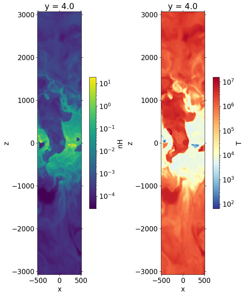
slc = ds.get_slice('y', ['nH', 'T', 'pressure']) # x-z slices
slc
<xarray.Dataset>
Dimensions:   (z: 768, x: 128)
Coordinates:
  * x         (x) float64 -508.0 -500.0 -492.0 -484.0 ... 492.0 500.0 508.0
    y         float64 4.0
  * z         (z) float64 -3.068e+03 -3.06e+03 -3.052e+03 ... 3.06e+03 3.068e+03
Data variables:
    pressure  (z, x) float32 2.693 2.68 2.657 2.631 ... 11.88 11.52 11.16 10.87
    nH        (z, x) float32 0.0001072 0.0001052 ... 0.0004483 0.0004352
    T         (z, x) float32 1.855e+06 1.881e+06 ... 1.839e+06 1.844e+06
Attributes:
    all_grid_equal:  True
    num:             200
    ngrid:           384
    le:              [ -512.  -512. -3072.]
    re:              [ 512.  512. 3072.]
    dx:              [8. 8. 8.]
    Lx:              [1024. 1024. 6144.]
    center:          [0. 0. 0.]
    Nx:              [128 128 768]
    ndim:            3
    time:            200.0007
dfi: {'rho': {'field_dep': ['density'], 'func': <function set...type(slc), type(slc.nH), type(slc.nH.data)
(xarray.core.dataset.Dataset, xarray.core.dataarray.DataArray, numpy.ndarray)
fig, axes = plt.subplots(1, 2, figsize=(8, 12), constrained_layout=True)
im1 = slc['nH'].plot(ax=axes[0], norm=LogNorm())
im2 = slc['T'].plot(ax=axes[1], norm=LogNorm(), cmap=cmap_temp)
for im in (im1, im2):
    im.axes.set_aspect('equal')
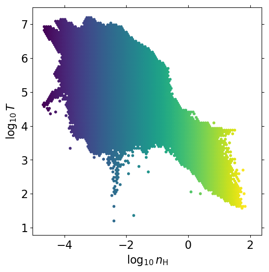
2d histogram#
lognH = np.log10(dat['nH'].data.flatten())
logT = np.log10(dat['T'].data.flatten())
# mass-weighted histograms
wgt = dat['nH'].data.flatten()
plt.hexbin(lognH, logT, wgt, mincnt=1, norm=mpl.colors.LogNorm())
plt.xlabel(r'$\log_{10}\,n_{\rm H}$')
plt.ylabel(r'$\log_{10}\,T$')
Text(0, 0.5, '$\\log_{10}\\,T$')
Plot projection and star particles#
sp = s.load_starpar_vtk(num=s.nums_starpar[0])
sp.columns
[LoadSim-INFO] [load_starpar_vtk]: R8_8pc_NCR.0200.starpar.vtk. Time: 200.000700
Index(['id', 'flag', 'n_ostar', 'mass', 'age', 'mage', 'metal_mass[0]',
       'metal_mass[1]', 'metal_mass[2]', 'metal_mass[3]', 'metal_mass[4]',
       'x1', 'x2', 'x3', 'v1', 'v2', 'v3'],
      dtype='object')
sp
| id | flag | n_ostar | mass | age | mage | metal_mass[0] | metal_mass[1] | metal_mass[2] | metal_mass[3] | metal_mass[4] | x1 | x2 | x3 | v1 | v2 | v3 | |
|---|---|---|---|---|---|---|---|---|---|---|---|---|---|---|---|---|---|
| 0 | 0 | -2 | 0 | 1.517063e+05 | 231.347687 | 231.347687 | 0.0 | 0.0 | 0.0 | 0.0 | 0.0 | -128.291458 | -450.330017 | 34.969208 | -3.673561 | -0.497162 | 2.552266 |
| 1 | 1 | -2 | 0 | 1.142920e+05 | 200.281982 | 200.281982 | 0.0 | 0.0 | 0.0 | 0.0 | 0.0 | -451.638062 | 448.136475 | 1.251051 | -1.985113 | 13.861067 | -0.561060 |
| 2 | 2 | -2 | 0 | 1.029942e+06 | 219.190628 | 219.190628 | 0.0 | 0.0 | 0.0 | 0.0 | 0.0 | -352.151489 | -204.598938 | 3.780031 | 5.817396 | 9.692892 | -1.035785 |
| 3 | 3 | -2 | 0 | 2.885881e+05 | 236.061691 | 236.061691 | 0.0 | 0.0 | 0.0 | 0.0 | 0.0 | -46.320374 | 399.499939 | -45.633480 | 1.270643 | 1.333141 | 7.092731 |
| 4 | 4 | -2 | 0 | 8.737053e+04 | 224.225128 | 224.225128 | 0.0 | 0.0 | 0.0 | 0.0 | 0.0 | -169.073090 | -75.030182 | -7.814175 | 9.002285 | 5.097887 | -2.412747 |
| ... | ... | ... | ... | ... | ... | ... | ... | ... | ... | ... | ... | ... | ... | ... | ... | ... | ... |
| 264 | 3619 | -1 | 0 | 0.000000e+00 | -9.412859 | 12.259128 | 0.0 | 0.0 | 0.0 | 0.0 | 0.0 | -17.949648 | -436.911743 | 68.887535 | 14.285395 | 42.216995 | 70.368149 |
| 265 | 3620 | -1 | 0 | 0.000000e+00 | -0.123773 | 4.554963 | 0.0 | 0.0 | 0.0 | 0.0 | 0.0 | 250.112442 | 487.829712 | -12.737943 | -6.930785 | -8.410844 | 22.714880 |
| 266 | 3621 | -1 | 0 | 0.000000e+00 | -24.058840 | 4.369840 | 0.0 | 0.0 | 0.0 | 0.0 | 0.0 | -214.895584 | -250.390366 | -6.121937 | -21.697975 | 38.959778 | -75.154793 |
| 267 | 3622 | -1 | 0 | 0.000000e+00 | -15.175461 | 12.259128 | 0.0 | 0.0 | 0.0 | 0.0 | 0.0 | -19.128952 | -454.030334 | 57.308399 | 13.182298 | -40.273441 | 46.820534 |
| 268 | 3623 | -1 | 0 | 0.000000e+00 | -1.964489 | 25.226053 | 0.0 | 0.0 | 0.0 | 0.0 | 0.0 | 72.532875 | -66.833473 | 8.098772 | 2.340160 | -29.183071 | 6.838042 |
269 rows × 17 columns
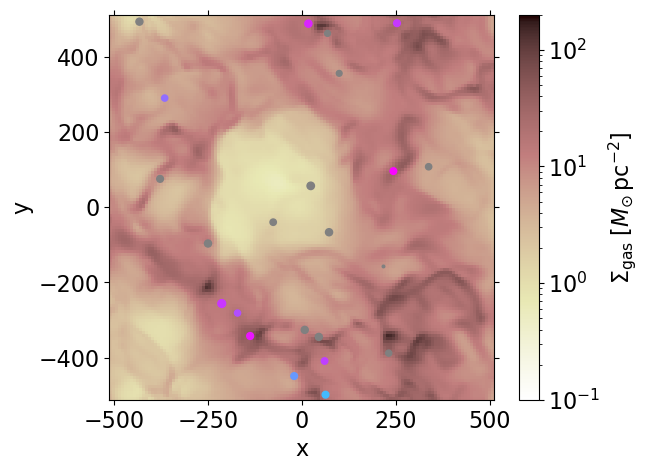
from pyathena.plt_tools.plt_starpar import scatter_sp

fig, ax = plt.subplots(1, 1, figsize=(6.5, 5))
d = ds.get_field('rho')
conv_Sigma = (1.0*au.g/au.cm**2).to('Msun pc-2').value
dz_cgs = ds.domain['dx'][2]*u.length.cgs.value

(d['rho'].sum(dim='z')*dz_cgs*conv_Sigma).plot.imshow(ax=ax,
    cmap='pink_r', norm=mpl.colors.LogNorm(0.1, 2e2),
    cbar_kwargs=dict(label=r'$\Sigma_{\rm gas}\;[M_{\odot}\,{\rm pc}^{-2}]$'))
ax.set_aspect('equal')

# Plot projected positions of star particles
# age < agemax : colored circles
# agemax < age_Myr < agemax_sn : grey circles
# with agemax = 20 Myr ; agemax_sn = 40Myr
scatter_sp(sp, ax, dim='z')
LoadSimTIGRESSNCR class#
For TIGRESS-classic and TIGRESS-NCR simulations, many derived information (such as total luminosity, number of sources) are calculated in pyathena/tigress_ncr/starpar.py
from pyathena.tigress_ncr.load_sim_tigress_ncr import LoadSimTIGRESSNCR

s = LoadSimTIGRESSNCR(basedir)
# s.print_all_properties()
Suppress warning
s.verbose = 'ERROR'
If you do not have permission to basedir, save pickles to a different directory, e.g., /home/USERNAME/basename/
s.savdir = os.path.join(os.path.expanduser('~'), s.basename)
star = s.read_starpar_all(force_override=True, savdir=s.savdir)
star.keys()
Index(['time', 'nstars', 'isrc', 'nsrc', 'sp_src', 'z_max', 'z_min',
       'z_mean_mass', 'z_mean_Qi', 'z_mean_LFUV', 'stdz_mass', 'stdz_Qi',
       'stdz_LFUV', 'Qi_tot', 'L_LW_tot', 'L_PE_tot', 'L_FUV_tot', 'Phi_i',
       'Sigma_FUV', 'sp'],
      dtype='object')
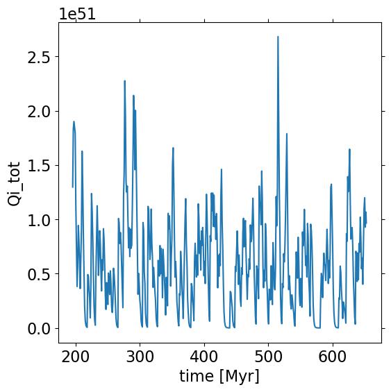
plt.plot(star['time']*s.u.Myr, star['Qi_tot']) # Total ionizing photon rate [1/s]
plt.setp(plt.gca(), xlabel='time [Myr]', ylabel='Qi_tot')
[Text(0.5, 0, 'time [Myr]'), Text(0, 0.5, 'Qi_tot')]
History dump#
# Read raw hst dump
h = pa.read_hst(s.files['hst']) # returns a pandas DataFrame object
h.columns
Index(['time', 'dt', 'mass', 'totalE', 'x1Mom', 'x2Mom', 'x3Mom', 'x1KE',
       'x2KE', 'x3KE', 'x1ME', 'x2ME', 'x3ME', 'gravPE', 'scalar0', 'scalar1',
       'scalar2', 'scalar3', 'scalar4', 'dmasssink', 'dM1sink', 'dM2sink',
       'dM3sink', 'dEsink', 'heat_ratio', 'heat_ratio_mid',
       'heat_ratio_mid_2p', 'ftau', 'x2dke', 'nmid', 'Pth_mid', 'Pturb_mid',
       'Vmid_2p', 'nmid_2p', 'Pth_mid_2p', 'Pturb_mid_2p', 'sfr10', 'sfr40',
       'sfr100', 'msp', 'metal_sp', 'total_ecool', 'total_eheat', 'total_enet',
       'V_Erad_PH', 'Lmasked_HI_PH', 'Lmasked_H2_PH', 'Lmasked_dust_PH',
       'Lmasked_dust_LW', 'Lmasked_dust_PE', 'phot_rate_HI', 'phot_rate_H2',
       'rec_rate_rad_HII', 'rec_rate_gr_HII', 'xi_CR0', 'Ltot0', 'Ltot1',
       'Ltot2', 'Ltot3', 'Lesc0', 'Lesc1', 'Lesc2', 'Lesc3', 'Ldust0',
       'Ldust1', 'Ldust2', 'Ldust3', 'Lxymax0', 'Lxymax1', 'Lxymax2',
       'Lxymax3', 'Lpp0', 'Lpp1', 'Lpp2', 'Lpp3'],
      dtype='object')
h.head()
| time | dt | mass | totalE | x1Mom | x2Mom | x3Mom | x1KE | x2KE | x3KE | ... | Ldust2 | Ldust3 | Lxymax0 | Lxymax1 | Lxymax2 | Lxymax3 | Lpp0 | Lpp1 | Lpp2 | Lpp3 | |
|---|---|---|---|---|---|---|---|---|---|---|---|---|---|---|---|---|---|---|---|---|---|
| 0 | 200.000700 | 0.002155 | 0.052018 | 24.523072 | -0.010668 | -0.114090 | 0.149412 | 2.067014 | 3.001098 | 3.706466 | ... | 2.404333e+12 | 653.116688 | 4.696874e+09 | 1.815048e+09 | 2.867097e+10 | 5.840392e+11 | 0.0 | 2.298291e+11 | 1.069728e+12 | 2.893340e+12 |
| 1 | 200.011568 | 0.002198 | 0.052018 | 24.417614 | -0.010663 | -0.114099 | 0.149376 | 2.056071 | 2.992799 | 3.695838 | ... | 2.404154e+12 | 653.411037 | 4.695982e+09 | 1.814261e+09 | 2.866940e+10 | 5.840334e+11 | 0.0 | 2.299529e+11 | 1.069950e+12 | 2.893498e+12 |
| 2 | 200.020375 | 0.002232 | 0.052018 | 24.338644 | -0.010658 | -0.114106 | 0.149347 | 2.047250 | 2.986004 | 3.686907 | ... | 2.398275e+12 | 650.927607 | 4.816156e+09 | 1.817778e+09 | 2.867580e+10 | 5.828847e+11 | 0.0 | 2.297048e+11 | 1.068698e+12 | 2.887522e+12 |
| 3 | 200.031582 | 0.002255 | 0.052018 | 24.242892 | -0.010653 | -0.114116 | 0.149309 | 2.036098 | 2.977272 | 3.675242 | ... | 2.391494e+12 | 648.406112 | 4.969366e+09 | 1.817014e+09 | 2.865399e+10 | 5.816466e+11 | 0.0 | 2.297736e+11 | 1.068160e+12 | 2.881460e+12 |
| 4 | 200.040671 | 0.002297 | 0.052018 | 24.166606 | -0.010648 | -0.114124 | 0.149279 | 2.027186 | 2.970138 | 3.665638 | ... | 2.391494e+12 | 648.406112 | 4.969366e+09 | 1.817014e+09 | 2.865399e+10 | 5.816466e+11 | 0.0 | 2.297736e+11 | 1.068160e+12 | 2.881460e+12 |
5 rows × 75 columns
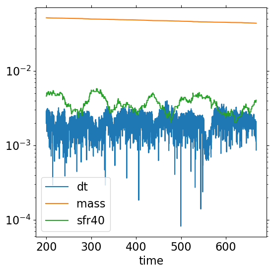
Plot
timestep size
dt_mhd(code unit)(total gas mass)/(volume of box) (code units)
\(\Sigma_{\rm SFR,40 Myr}\) (Msun/yr/kpc^2)
ax = h.plot('time', y=['dt','mass', 'sfr40'])
ax.set_yscale('log')
Read history dump post-processed (and saved to a pickle) using the script pyathena/tigress_ncr/hst.py
h = s.read_hst()
h.columns
Index(['time_code', 'time', 'time_orb', 'dt_code', 'dt', 'mass', 'mass_sp',
       'mass0', 'mass1', 'mass2', 'mass3', 'mass4', 'M_HI', 'Sigma_HI', 'M_H2',
       'Sigma_H2', 'M_HII', 'Sigma_HII', 'massflux_lbd_d', 'massflux_ubd_d',
       'mass_out', 'Sigma_gas', 'Sigma_sp', 'Sigma_out', 'mass_snej',
       'Sigma_snej', 'H', 'mf_c', 'vf_c', 'H_c', 'mf_u', 'vf_u', 'H_u',
       'mf_w1', 'vf_w1', 'H_w1', 'mf_w2', 'vf_w2', 'H_w2', 'mf_h1', 'vf_h1',
       'H_h1', 'mf_h2', 'vf_h2', 'H_h2', 'mf_w', 'vf_w', 'H_w', 'mf_2p',
       'vf_2p', 'H_2p', 'KE', 'ME', 'v1', 'vA1', 'v1_2p', 'v2', 'vA2', 'v2_2p',
       'v3', 'vA3', 'v3_2p', 'cs', 'Pth_mid', 'Pth_mid_2p', 'Pturb_mid',
       'Pturb_mid_2p', 'nmid', 'nmid_2p', 'sfr10', 'sfr40', 'sfr100',
       'Ltot_PH', 'Lesc_PH', 'Ldust_PH', 'Qtot_PH', 'Qesc_PH', 'Qtot_cum_PH',
       'Qesc_cum_PH', 'fesc_PH', 'fesc_cum_PH', 'Ltot_LW', 'Lesc_LW',
       'Ldust_LW', 'Qtot_LW', 'Qesc_LW', 'Qtot_cum_LW', 'Qesc_cum_LW',
       'fesc_LW', 'fesc_cum_LW', 'Ltot_PE', 'Lesc_PE', 'Ldust_PE', 'Qtot_PE',
       'Qesc_PE', 'Qtot_cum_PE', 'Qesc_cum_PE', 'fesc_PE', 'fesc_cum_PE',
       'xi_CR0'],
      dtype='object')