Starburst99: Stellar Population Synthesis

This notebook demonstrates the pyathena.util.sb99 module, which reads and analyses output from the Starburst99 stellar population synthesis code.

We use a solar-metallicity (\(Z = 0.014\)), instantaneous-burst cluster of \(10^6\,M_\odot\) with Geneva standard tracks (no rotation; Leitherer et al. 1999).

Dataset note: Two bundled datasets are stored under data/sb99/, with .spectrum1 files compressed as .bz2 to reduce size:

• Z014_M1E6_GenevaV00_dt02/ — sub-sampled from a full Starburst99 run with uniform \(\Delta t = 0.1\) Myr (1000 steps, 0–100 Myr) to 251 uniform steps at \(\Delta t = 0.2\) Myr (0–50 Myr). Used for this notebook.

• Z014_M1E6_GenevaV00_logdt_10Gyr/ — sub-sampled from a log-spaced Starburst99 run (378 steps, 2 Myr–10 Gyr) to 77 log-spaced steps. Used together with the above for ISRF calculations (sb99.get_ISRF_SB99_plane_parallel).

All other output files (.power1, .snr1, etc.) are copied from the original runs without modification.

Topics covered:

1. Loading SB99 data

2. SED evolution

3. Band-integrated luminosities and momentum injection rates

4. Dust cross sections and mean photon energies vs age

5. Supernova and stellar wind feedback

import os
import numpy as np
import matplotlib.pyplot as plt
import astropy.units as au
import astropy.constants as ac

import pyathena as pa
from pyathena.util import sb99
from pyathena.plt_tools.set_plt import set_plt_fancy

set_plt_fancy()

# Path to the bundled SB99 dataset
import pathlib
REPO = pathlib.Path(pa.__file__).parent.parent
BASEDIR = REPO / 'data' / 'sb99' / 'Z014_M1E6_GenevaV00_dt02'

1. Load SB99 data

SB99 discovers the output files automatically from the directory.

sb = sb99.SB99(str(BASEDIR), verbose=True)

rr = sb.read_rad()    # radiation output
rw = sb.read_wind()   # stellar wind power and momentum
rs = sb.read_sn()     # supernova rate and energy

[SB99-INFO] basedir: /Users/jgkim/Dropbox/Projects/pyathena/data/sb99/Z014_M1E6_GenevaV00_dt02

[SB99-INFO] Fixed mass; logM: 6.00, tmax: 100.0 Myr

[SB99-INFO] IMF: 2 interval(s), exponents=[1.3, 2.3], mass limits=[0.1, 0.5, 100.0] Msun

[SB99-INFO] Tracks: GENEVA v00 (IZ=54, Z=0.014); SN cutoff: 8 Msun; wind model: 0 (Maeder)

[SB99-INFO] Time range: 0.01 – 50.0 Myr  (251 steps)

[SB99-INFO] Wavelength range: 91 – 1600000 Å  (1221 points)

[SB99-INFO] Band luminosity keys: ['tot', 'LyC', 'LW', 'PE', 'OPT', 'IR', 'FUV', 'UV']

[SB99-INFO] Wind: time 0.01–99.9 Myr  (1000 steps); peak Edot_all 5.28e+00 Lsun Msun-1 at 3.2 Myr

[SB99-INFO] SN: time 0.01–99.9 Myr  (1000 steps); peak rate 5.93e-10 yr-1 Msun-1 at 4.7 Myr

Return fields of read_rad()

read_rad() returns a dictionary rr with the following keys:

Key	Type	Description
time_Myr, time_yr	1-D array (ntime,)	Stellar population age [Myr, yr]
wav	1-D array (nwav,)	Wavelength grid [Å]
logf	2-D array (ntime, nwav)	\(\log_{10} L_\lambda\) [erg s\(^{-1}\) Å\(^{-1}\)] for the full cluster of mass \(10^{\rm logM}\,M_\odot\). Specific luminosity per \(M_\odot\): 10**(logf - logM)
logM	float	\(\log_{10}\) cluster mass [\(M_\odot\)]
df	DataFrame	Raw per-timestep spectral table with columns time_Myr, wav, logf, logfstar, logfneb
L	dict of arrays	Specific luminosity [\(L_\odot\,M_\odot^{-1}\)]; keys: 'tot', 'LyC', 'LW', 'PE', 'FUV', 'OPT', 'IR'
pdot	dict of arrays	Specific radiation momentum rate [\(M_\odot\,\mathrm{km\,s^{-1}\,Myr^{-1}}\,M_\odot^{-1}\)]; same keys as L
Q	dict of arrays	Specific ionizing-photon rate [s\(^{-1}\,M_\odot^{-1}\)]; same keys as L
Cext, Cabs, Crpr	dict of arrays	Luminosity-weighted mean dust cross sections per H nucleon [cm\(^2\) H\(^{-1}\)]
hnu	dict of arrays	Luminosity-weighted mean photon energy [eV]
sigma_pi_H, sigma_pi_H2	array	Luminosity-weighted mean PI cross section for H and H\(_2\) [cm\(^2\)]
dhnu_H_LyC, dhnu_H2_LyC	array	Mean excess photon energy above ionization threshold for H and H\(_2\) [eV]
tdecay_lum	dict	Luminosity-weighted mean emission time [Myr]
tcumul_lum_50/90	dict	Age at which 50%/90% of cumulative band luminosity is emitted [Myr]
*_avg, *_Lavg, *_Qavg	dict	Time-, \(L\)-, and \(Q\)-weighted cumulative running averages

2. SED evolution

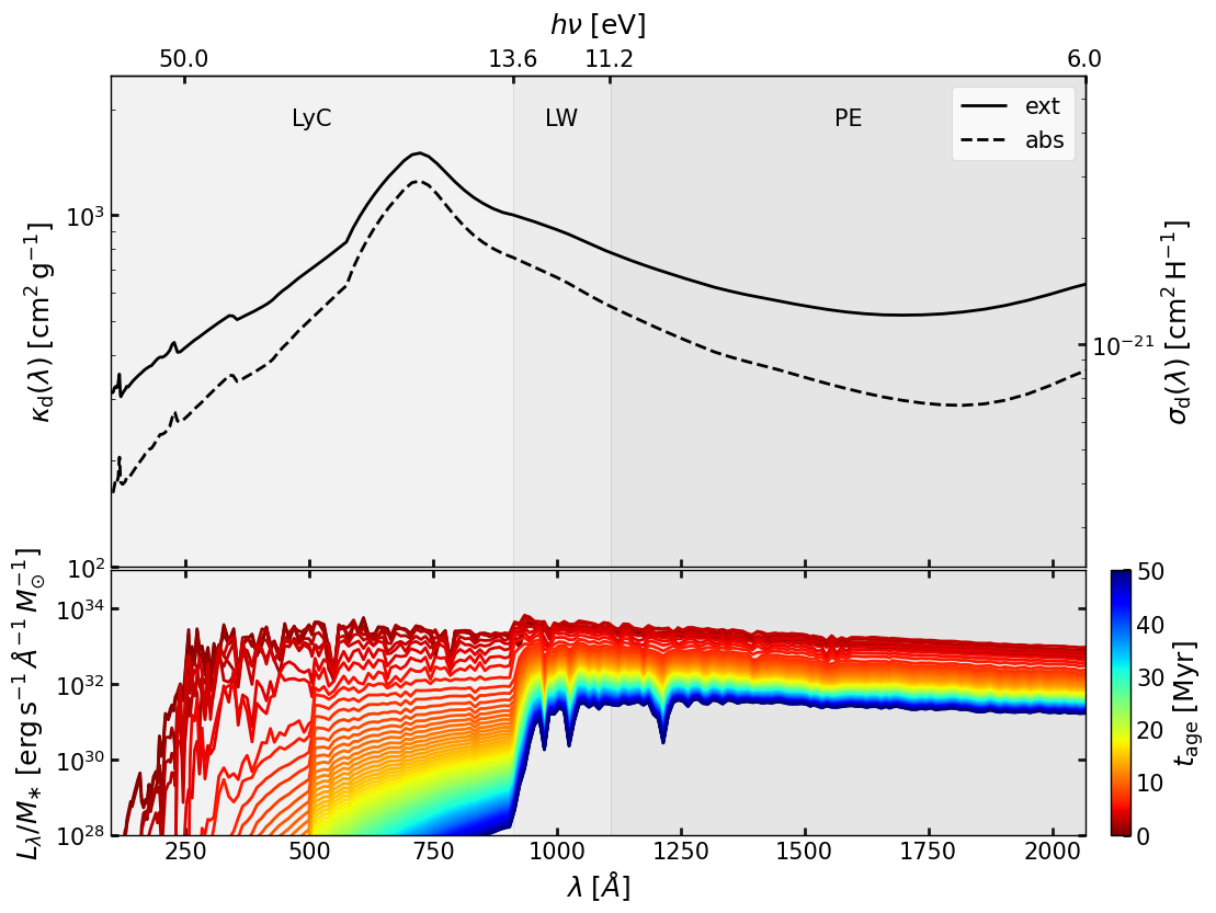
The figure has two panels:

• Top: Dust extinction (\(C_{\rm ext}/\mu_H\), solid) and absorption (\(\kappa_{\rm abs}\), dashed) cross sections per unit gas mass as a function of wavelength, from the Weingartner & Draine (2001) dust model (\(R_V = 3.1\)).

• Bottom: \(L_\lambda / M_*\) as a function of wavelength at different ages, color-coded from blue (young) to red (old). Grey bands mark the LyC (\(<912\,\text{Å}\)), LW (\(912–1108\,\text{Å}\)), and PE (\(1108–2068\,\text{Å}\)) bands used for band integration.

fig = sb.plt_spec_sigmad(rr, tmax=50.0, nstride=3, plt_isrf=False)

0.0 0.6 1.2 1.8 2.4 3.0 3.6 4.2 4.8 5.4 6.0 6.6 7.2 7.8 8.4 9.0 9.6 10.2 10.8 11.4 12.0 12.6 13.2 13.8 14.4 15.0 15.6 16.2 16.8 17.4 18.0 18.6 19.2 19.8 20.4 21.0 21.6 22.2 22.8 23.4 24.0 24.6 25.2 25.8 26.4 27.0 27.6 28.2 28.8 29.4 30.0 30.6 31.2 31.8 32.4 33.0 33.6 34.2 34.8 35.4 36.0 36.6 37.2 37.8 38.4 39.0 39.6 40.2 40.8 41.4 42.0 42.6 43.2 43.8 44.4 45.0 45.6 46.2 46.8 47.4 48.0 48.6 49.2 49.8 

/Users/jgkim/Dropbox/Projects/pyathena/pyathena/util/sb99.py:753: RuntimeWarning: divide by zero encountered in divide
  return 1.0/(ac.h.cgs.value*ac.c.cgs.value/1e-8/(1.0*au.eV).cgs.value)/x

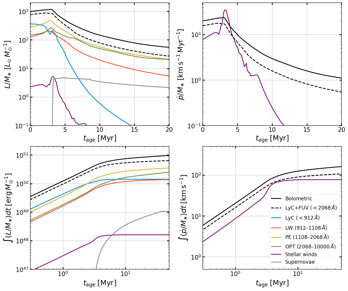
3. Band-integrated luminosity and momentum vs age

fig, axes = plt.subplots(2, 2, figsize=(12, 10), constrained_layout=True,
                         gridspec_kw=dict(height_ratios=[0.5, 0.5]))
axes = axes.flatten()

sb.plt_lum_evol(axes[0], rr, rw, rs, plt_sn=True)
sb.plt_pdot_evol(axes[1], rr, rw, rs)
sb.plt_lum_cumul(axes[2], rr, rw, rs, normed=False, plt_sn=True)
sb.plt_pdot_cumul(axes[3], rr, rw, rs, normed=False)

for ax in axes:
    ax.grid()

import matplotlib as mpl
plt.legend(
    [mpl.lines.Line2D([0],[0],c='k'),
     mpl.lines.Line2D([0],[0],c='k',ls='--'),
     mpl.lines.Line2D([0],[0],c='C0'),
     mpl.lines.Line2D([0],[0],c='C1'),
     mpl.lines.Line2D([0],[0],c='C2'),
     mpl.lines.Line2D([0],[0],c='C3'),
     mpl.lines.Line2D([0],[0],c='C7'),
     mpl.lines.Line2D([0],[0],c='C8')],
    ['Bolometric', r'LyC+FUV ($<2068\,\AA$)',
     r'LyC ($<912\,\AA$)', r'LW ($912$–$1108\,\AA$)',
     r'PE ($1108$–$2068\,\AA$)', r'OPT ($2068$–$10000\,\AA$)',
     'Stellar winds', 'Supernovae'],
    loc=4, fontsize='small')

plt.show()

Luminosity-weighted timescales

The luminosity-weighted decay timescale \(t_{\rm decay} = \int L\,t\,dt / \int L\,dt\) and the times by which 50% and 90% of the cumulative energy has been emitted.

print('{:<6s}  {:>12s}  {:>14s}  {:>14s}'.format(
    'Band', 't_decay (Myr)', 't_cumul_50 (Myr)', 't_cumul_90 (Myr)'))
print('-' * 52)
for k in ['LyC', 'LW', 'PE', 'FUV', 'OPT', 'tot']:
    print('{:<6s}  {:>12.1f}  {:>14.1f}  {:>14.1f}'.format(
        k,
        rr['tdecay_lum'][k],
        rr['tcumul_lum_50'][k],
        rr['tcumul_lum_90'][k]))

Band    t_decay (Myr)  t_cumul_50 (Myr)  t_cumul_90 (Myr)
----------------------------------------------------
LyC              1.9             1.6             3.8
LW               5.9             3.4            13.6
PE               8.1             4.0            22.6
FUV              7.5             3.8            20.0
OPT             11.5             6.0            32.8
tot              8.0             3.6            23.2

Accessing band-integrated luminosities

The rr['L'] dictionary stores luminosity per solar mass (erg s\(^{-1}\) M\(_{\odot}^{-1}\)) as a function of time for each band. Below is a minimal example.

Mcluster = 1e6  # Msun
t = rr['time_Myr']         # shape (N_time,)
L_LyC = rr['L']['LyC']    # L_sun/Msun, shape (N_time,)

# Luminosity at a specific age
i3 = np.argmin(np.abs(t - 3.0))
print(f'LyC luminosity at t = {t[i3]:.1f} Myr: '
      f'{L_LyC[i3]*Mcluster:.2e} Lsun  (for {Mcluster:.1e} Msun cluster)')

# Peak luminosity
ipeak = np.argmax(L_LyC)
print(f'Peak LyC luminosity:            {L_LyC[ipeak]*Mcluster:.2e} Lsun  at t = {t[ipeak]:.1f} Myr')

LyC luminosity at t = 3.0 Myr: 1.81e+08 Lsun  (for 1.0e+06 Msun cluster)
Peak LyC luminosity:            3.62e+08 Lsun  at t = 0.0 Myr

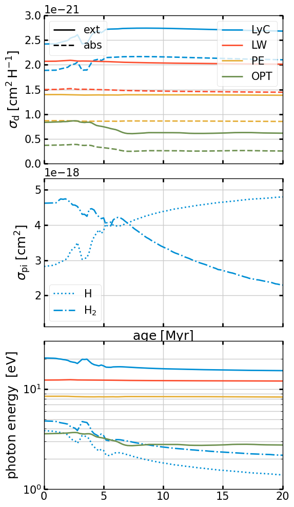
4. Dust cross sections and mean photon energies vs age

Luminosity-weighted mean dust extinction/absorption cross section per H atom (\(\langle \sigma_d \rangle\)), photoionization cross sections for H and H\(_2\) (\(\langle \sigma_{\rm pi} \rangle\)), and mean photon energies (\(\langle h\nu \rangle\)) as a function of stellar age for each radiation band.

fig = sb99.plt_cross_sections_hnu(rr)

Time-averaged values (first 20 Myr)

Print luminosity- and photon-rate-weighted averages of cross sections and mean photon energies over the first 20 Myr.

sb99.print_lum_weighted_avg_quantities(rr, tmax=20.0)

Luminosity-weighted timescale int t*L dt/int L dt: {'tot': 8.033181841634132, 'LyC': 1.9362249576881663, 'LW': 5.872428114864254, 'PE': 8.121941423868194, 'OPT': 11.525287455130114, 'IR': 15.705568862708475, 'FUV': 7.4804580606224516, 'UV': 6.244589339918595}
Bolometric at t=0: 985.5964350981222 1165.8656320873888 3.01
Bolometric at maximum: 1165.8656320873888
Time at maximum of Bolometric: 3.01
Lyman Continuum
- 50% of LyC photons are emitted in the first 1.61 Myr
- 90% of LyC photons are emitted in the first 3.81 Myr
- 95% of LyC photons are emitted in the first 4.41 Myr
- 50% of the initial value at 2.81 Myr
FUV (LW+PE)
- 50% of FUV photons are emitted in the first 3.81 Myr
- 90% of FUV photons are emitted in the first 20.01 Myr
- 95% of FUV photons are emitted in the first 30.21 Myr
- 50% of the initial value at 6.21 Myr
LyC :
Cabs Cext Crpr hnu : 1.94e-21, 2.48e-21, 2.10e-21 1.95e+01
sigma_pi_H dhnu_H 3.08e-18, 3.46e+00
sigma_pi_H2 dhnu_H2 4.56e-18, 4.46e+00
LW :
Cabs Cext Crpr hnu : 1.50e-21, 2.07e-21, 1.69e-21 1.22e+01
PE :
Cabs Cext Crpr hnu : 8.61e-22, 1.39e-21, 1.05e-21 8.39e+00
OPT :
Cabs Cext Crpr hnu : 3.22e-22, 7.47e-22, 5.17e-22 3.24e+00

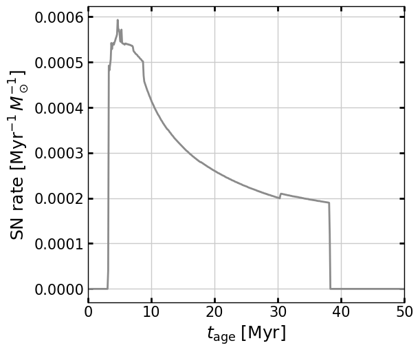
5. Supernova and wind feedback

fig, ax = plt.subplots(figsize=(6, 5), constrained_layout=True)

ax.plot(rs['time_Myr'], rs['SN_rate']*1e6, c='C8')
ax.set_xlabel(r'$t_{\rm age}\;[{\rm Myr}]$')
ax.set_ylabel(r'SN rate $[{\rm Myr}^{-1}\,M_\odot^{-1}]$')
ax.set_xlim(0, 50)
ax.grid()
plt.show()

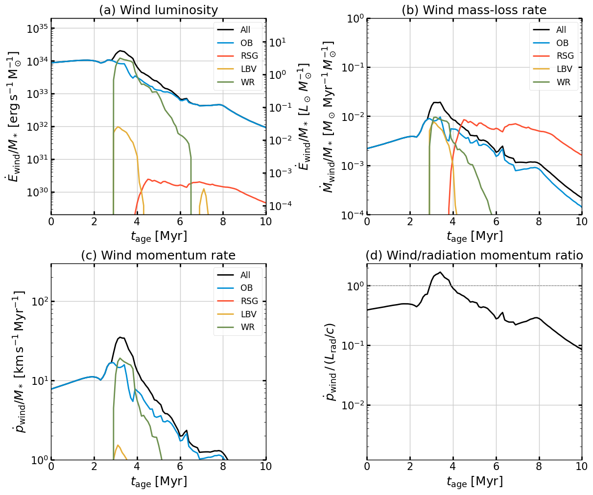
Stellar wind feedback

Evolution of key wind quantities per unit stellar mass as computed by Starburst99 (Leitherer et al. 1999): (a) wind luminosity, (b) wind mass-loss rate, (c) wind momentum injection rate, and (d) ratio of wind to radiation momentum injection rate.

from scipy.interpolate import interp1d

Lsun = ac.L_sun.cgs.value
clight = ac.c.cgs.value
# pdot_wind unit in rw: Msun km/s/Myr/Msun  -->  dyne/Msun
pdot_conv = (1.0*au.Msun*au.km/au.s/au.Myr).to('dyne').value

fig, axes = plt.subplots(2, 2, figsize=(12, 10), constrained_layout=True)
axes = axes.flatten()

components = [('all','k','All'), ('OB','C0','OB'),
              ('RSG','C1','RSG'), ('LBV','C2','LBV'), ('WR','C3','WR')]

# (a) Wind luminosity [erg/s/Msun], right axis [Lsun/Msun]
ax = axes[0]
for v, c, label in components:
    ax.semilogy(rw['time_Myr'], rw[f'Edot_{v}'], c=c, label=label)
ymax = rw['Edot_all'].max()
ax.set_ylim(ymax*1e-5, ymax*10)
ax2 = ax.twinx()
ax2.set_yscale('log')
ax2.set_ylim(ax.get_ylim()[0]/Lsun, ax.get_ylim()[1]/Lsun)
ax2.set_ylabel(r'$\dot{E}_{\rm wind}/M_*\;[L_\odot\,M_\odot^{-1}]$')
ax.set_ylabel(r'$\dot{E}_{\rm wind}/M_*\;[{\rm erg\,s^{-1}\,M_\odot^{-1}}]$')
ax.legend(fontsize='small')
ax.set_title('(a) Wind luminosity')

# (b) Mass-loss rate [Msun/Myr/Msun]
ax = axes[1]
for v, c, label in components:
    ax.semilogy(rw['time_Myr'], rw[f'Mdot_{v}'], c=c, label=label)
ax.set_ylim(1e-4, 1e0)
ax.set_ylabel(r'$\dot{M}_{\rm wind}/M_*\;[M_\odot\,{\rm Myr}^{-1}\,M_\odot^{-1}]$')
ax.legend(fontsize='small')
ax.set_title('(b) Wind mass-loss rate')

# (c) Wind momentum rate [km/s/Myr]
#     pdot_all in rw is Msun km/s/Myr / Msun = km/s/Myr
ax = axes[2]
for v, c, label in components:
    ax.semilogy(rw['time_Myr'], rw[f'pdot_{v}'], c=c, label=label)
ax.set_ylim(1e0, 3e2)
ax.set_ylabel(r'$\dot{p}_{\rm wind}/M_*\;[{\rm km\,s^{-1}\,Myr^{-1}}]$')
ax.legend(fontsize='small')
ax.set_title('(c) Wind momentum rate')

# (d) Ratio pdot_wind / (L_rad/c)
#     rr['L']['tot'] is in Lsun/Msun; convert to erg/s/Msun before dividing by c
ax = axes[3]
L_tot_interp = interp1d(rr['time_Myr'], rr['L']['tot'],
                        bounds_error=False, fill_value='extrapolate')
L_rad_cgs = L_tot_interp(rw['time_Myr']) * Lsun  # erg/s/Msun
pdot_rad = L_rad_cgs / clight                      # dyne/Msun
pdot_wind_cgs = rw['pdot_all'] * pdot_conv
ratio = pdot_wind_cgs / pdot_rad
ax.semilogy(rw['time_Myr'], ratio, c='k')
ax.axhline(1, ls='--', c='gray', lw=0.8)
ax.set_ylabel(r'$\dot{p}_{\rm wind}\,/\,(L_{\rm rad}/c)$')
ax.set_title('(d) Wind/radiation momentum ratio')

for ax in axes:
    ax.set_xlabel(r'$t_{\rm age}\;[{\rm Myr}]$')
    ax.set_xlim(0, 10)
    ax.grid()

plt.show()

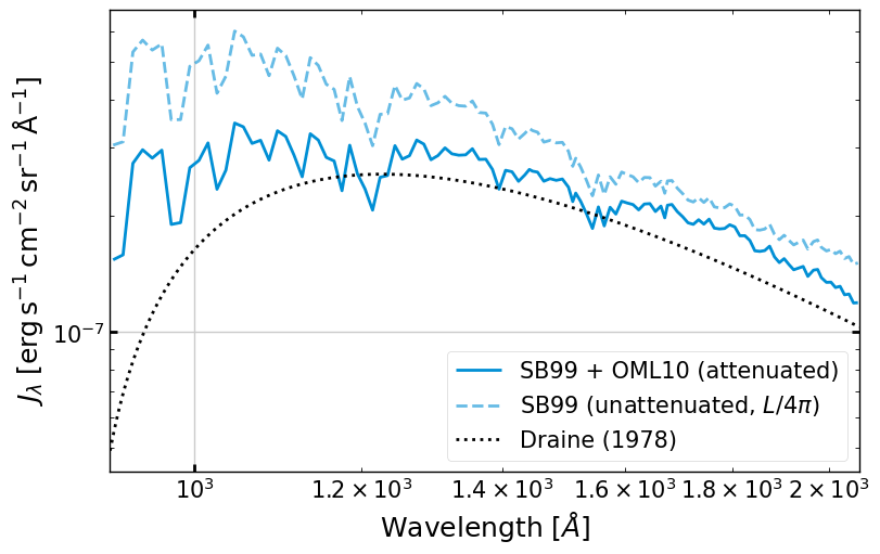
6. Interstellar Radiation Field (ISRF)

The function sb99.get_ISRF_SB99_plane_parallel estimates the angle-averaged mean intensity \(J_\lambda\) at the midplane of a plane-parallel disk under a constant star-formation history, following Ostriker et al. (2010):

\[J_\lambda = \frac{L_\lambda / {\rm SFR}}{4\pi} \cdot \Sigma_{\rm SFR} \cdot \frac{1 - E_2(\tau_\perp/2)}{\tau_\perp}\]

where \(\tau_\perp(\lambda)\) is the wavelength-dependent perpendicular dust optical depth and \(E_2\) is the second exponential integral.

By default the function stitches the fine-resolution short-timescale dataset (dt = 0.2 Myr, 0–50 Myr) with the log-spaced long-timescale dataset (2 Myr–10 Gyr) and integrates over a constant SFH up to \(t_{\rm max} = 10\) Gyr:

\[\frac{L_\lambda}{\rm SFR} = \int_0^{t_{\rm max}} \frac{L_\lambda^{\rm SSP}(t)}{M_*}\,dt\]

from pyathena.util import sb99
from pyathena.util.rad_isrf import nuJnu_Dr78

# Compute midplane ISRF for typical ISM conditions
r = sb99.get_ISRF_SB99_plane_parallel(
    Sigma_gas=10.0*au.M_sun/au.pc**2,
    Sigma_SFR=2.5e-3*au.M_sun/au.kpc**2/au.yr,
    verbose=False)

w = r['w_angstrom']
idx_fuv = (w > 912) & (w < 2068)

fig, ax = plt.subplots(figsize=(8, 5), constrained_layout=True)

# Attenuated and unattenuated midplane ISRF
l, = ax.loglog(w[idx_fuv], r['Jlambda'][idx_fuv],
               label=r'SB99 + OML10 (attenuated)')
ax.loglog(w[idx_fuv], r['Jlambda_unatt'][idx_fuv],
          c=l.get_color(), ls='--', alpha=0.6,
          label=r'SB99 (unattenuated, $L/4\pi$)')

# Draine (1978) reference ISRF
wav_dr = np.logspace(np.log10(912), np.log10(2068), 500)*au.angstrom
nu_dr  = (ac.c / wav_dr).to('Hz')
E_dr   = (nu_dr * ac.h).to('eV')
J_dr78 = nuJnu_Dr78(E_dr) / wav_dr   # nuJnu / lambda = J_lambda
ax.loglog(wav_dr.value, J_dr78.to('erg s-1 cm-2 angstrom-1 sr-1').value,
          c='k', ls=':', label='Draine (1978)')

ax.set_xlabel(r'Wavelength $[\AA]$')
ax.set_ylabel(r'$J_\lambda\;[{\rm erg\,s^{-1}\,cm^{-2}\,sr^{-1}\,\AA^{-1}}]$')
ax.set_xlim(912, 2068)
ax.legend()
ax.grid()
plt.show()

print(f"\nBand-integrated FUV mean intensity:")
print(f"  J_FUV (attenuated) : {r['J_FUV']:.3e}")
print(f"  J_FUV (unattenuated): {r['J_FUV_unatt']:.3e}")
print(f"  Attenuation factor  : {(r['J_FUV']/r['J_FUV_unatt']).decompose().value:.3f}")

Band-integrated FUV mean intensity:
  J_FUV (attenuated) : 2.596e-04 erg / (s sr cm2)
  J_FUV (unattenuated): 3.604e-04 erg / (s sr cm2)
  Attenuation factor  : 0.720